Plotting Plain Receiver Functions#
Single Receiver Function#
Given the data downloaded using the example notebook for data collection, we can simply read and plot them using
 1from pyglimer.rf.create import read_rf
 2set_mpl_params()
 3
 4# Read all RFs from Station IU/HRV
 5rfst = read_rf("../database/waveforms/RF/P/IU/HRV/*.sac")
 6
 7# Some random RF from the 800 avalable one at IU.HRV
 8N = 753
 9
10# Plot RF and save its output.
11rfst[N].plot()
which results in the following image:
We can time limit the figure as well
rfst[N].plot(tlim=[0, 20])
which cuts out the RF between 0 and 20 seconds
If you feel artsy and only want the trace
rfst[N].plot(tlim=[0, 20], clean=True)
which removes all labels, axes etc.
Refer to plot() and plot()
for all possible plotting arguments.
Receiver Function Section#
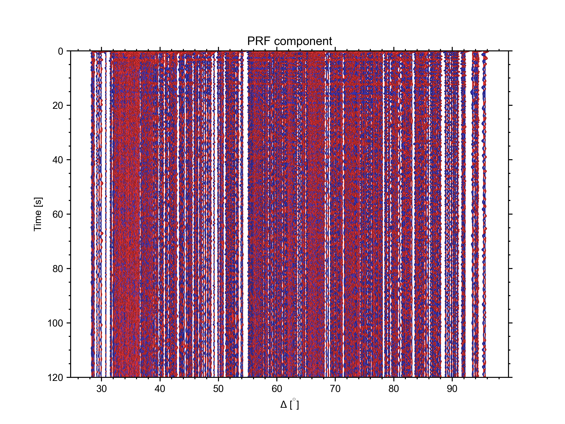
We can plot all receiver functions in an RFStream into a section depending
on epicentral distance.
# Plot section
rfst.plot(scalingfactor=1)
This plots all available RFs in the Stream into a section

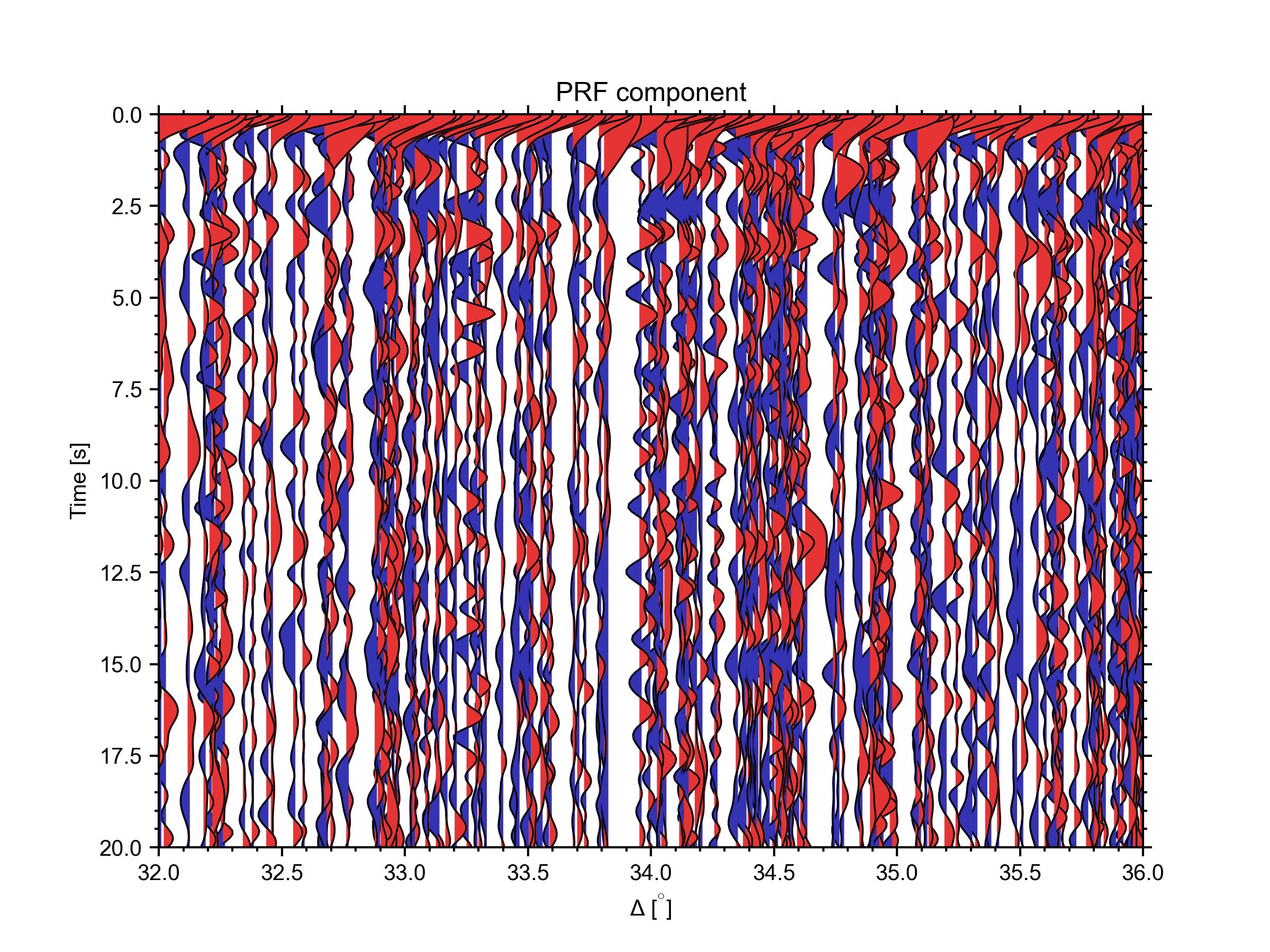
Also this plot can be limited using the right arguments
1# Plot section with limits
2timelimits = (0, 20)  # seconds
3epilimits = (32, 36)  # epicentral distance
4rfst.plot(
5    scalingfactor=0.25, linewidth=0.75,
6    timelimits=timelimits, epilimits=epilimits
7    )
which provides a more detailed view of the receiver functions
