HDF5 Database

This example is nearly identical to the MSEED tutorial except the fact that we are specifying a different data format in the request dictionary.

Downloading Event & Station Metadata

In this section, the only difference is the format key in the request_dict that is set to hdf5.

# sphinx_gallery_thumbnail_number = 1
# sphinx_gallery_dummy_images = 1

First let’s get a path where to create the data.

# Some needed Imports
import os
from typing import NewType
from obspy import UTCDateTime
from pyglimer.waveform.request import Request

# Get notebook path for future reference of the database:
# Get notebook path for future reference of the database:
try: db_base_path = ipynb_path
except NameError:
    try: db_base_path = os.path.dirname(os.path.realpath(__file__))
    except NameError: db_base_path = os.getcwd()

# Define file locations
proj_dir = os.path.join(db_base_path, 'tmp', 'database_hdf5')

# Define network and station to download RFs for
network = 'IU'
station = 'HRV'

request_dict = {
    # Necessary arguments
    'proj_dir': proj_dir,
    'raw_subdir': os.path.join('waveforms', 'raw'),# Directory of the waveforms
    'prepro_subdir': os.path.join('waveforms', 'preprocessed'),  # Directory of the preprocessed waveforms
    'rf_subdir': os.path.join('waveforms', 'RF'),  # Directory of the receiver functions
    'statloc_subdir': 'stations', # Directory stations
    'evt_subdir': 'events',       # Directory of the events
    'log_subdir': 'log',          # Directory for the logs
    'loglvl': 'WARNING',          # logging level
    'format': 'hdf5',              # Format to save database in
    "phase": "P",                 # 'P' or 'S' receiver functions
    "rot": "RTZ",                 # Coordinate system to rotate to
    "deconmeth": "waterlevel",    # Deconvolution method
    "starttime": UTCDateTime(2021, 1, 1, 0, 0, 0), # Starttime of database.
                                                # Here, starttime of HRV
    "endtime": UTCDateTime(2021, 7, 1, 0, 0, 0), # Endtimetime of database
    # kwargs below
    "pol": 'v',                   # Source wavelet polaristion. Def. "v" --> SV
    "minmag": 5.5,                # Earthquake minimum magnitude. Def. 5.5
    "event_coords": None,         # Specific event?. Def. None
    "network": network,              # Restricts networks. Def. None
    "station": station,             # Restricts stations. Def. None
    "waveform_client": ["IRIS"],  # FDSN server client (s. obspy). Def. None
    "evtcat": None,               # If you have already downloaded a set of
                                # events previously, you can use them here
}

Now that all parameters are in place, let’s initialize the pyglimer.waveform.request.Request

# Initializing the Request class and downloading the data
R = Request(**request_dict)

The initialization will look for all events for which data is available. To see whether the events make sense we plot a map of the events:

import matplotlib.pyplot as plt
from pyglimer.plot.plot_utils import plot_catalog
from pyglimer.plot.plot_utils import set_mpl_params

# Setting plotting parameters
set_mpl_params()

# Plotting the catalog
plot_catalog(R.evtcat)

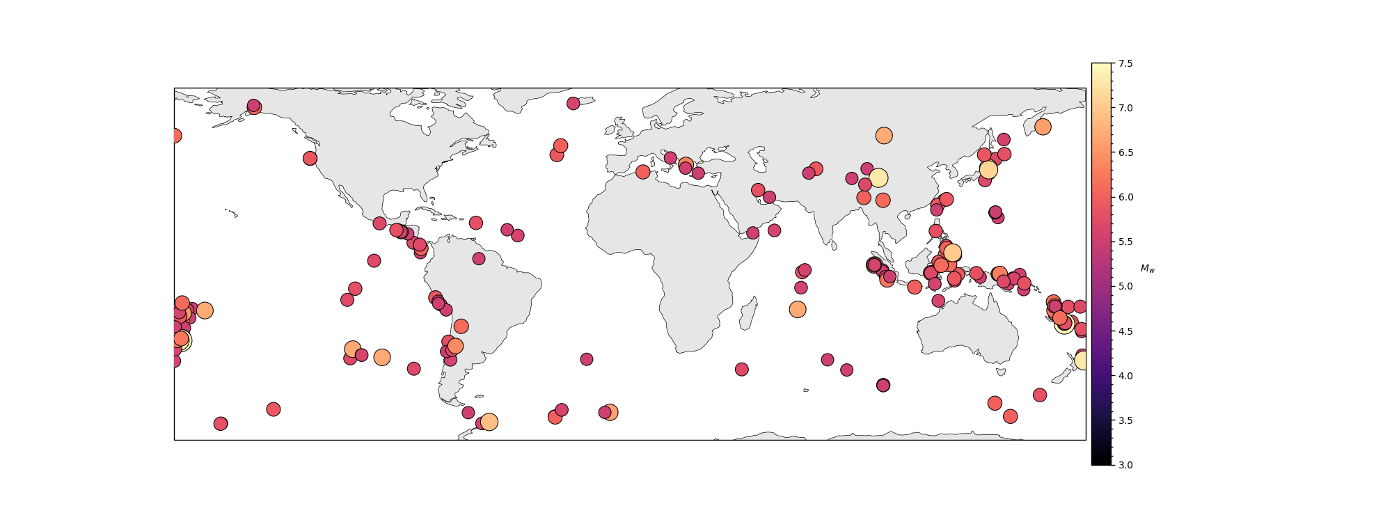
We can also quickly check how many events we gathered.

print(f"There are {len(R.evtcat)} available events")

There are 289 available events

---

Again, this section does not really change, because the request_dict parsed all needed information to pyglimer.waveform.request.Request.

R.download_waveforms_small_db(channel='BH?')

--> Enter TOA event loop for station IU.HRV

there is indeed a change in the code because we saved the raw data in form of ASDFDataset``s and we need to actually access the ``hdf5 file that we to count how many traces it contains.

# Import RawDataBase
from pyglimer.database.raw import RawDatabase

# Path to the where the miniseeds are stored
data_storage = os.path.join(
    proj_dir, 'waveforms', 'raw', 'P', f'{network}.{station}.h5')

# Read the data from the station ``h5`` file
with RawDatabase(data_storage, mode='r') as ds:

    # Perform waveform query on ASDFDataSet
    stream = ds.get_data(
        network,
        station,
        '*',  # Event ID
        'raw')

# Print output
print(f"Number of downloaded waveforms: {len(stream)}")

Number of downloaded waveforms: 207

The final step to get you receiver function data is the preprocessing. Although it is hidden in a single function, which is pyglimer.waveform.request.Request.preprocess() A lot of decisions are being made:

Processing steps: 1. Clips waveform to the right length (tz before and ta after theorethical arrival.) 2. Demean & Detrend 3. Tapering 4. Remove Instrument response, convert to velocity & simulate havard station 5. Rotation to NEZ and, subsequently, to RTZ. 6. Compute SNR for highpass filtered waveforms (highpass f defined in qc.lowco) If SNR lower than in qc.SNR_criteria for all filters, rejects waveform. 7. Write finished and filtered waveforms to folder specified in qc.outputloc. 8. Write info file with shelf containing station, event and waveform information. 9. (Optional) If we had chosen a different coordinate system in rot than RTZ, it would now cast the preprocessed waveforms information that very coordinate system. 10. Deconvolution with method deconmeth from our dict is perfomed.

R.preprocess(hc_filt=1.5, client='single')

  0%|          | 0/1 [00:00<?, ?it/s]

  0%|          | 0/289 [00:00<?, ?it/s]

  2%|2         | 6/289 [00:00<00:05, 47.69it/s]

  8%|7         | 23/289 [00:00<00:02, 101.87it/s]

 12%|#1        | 34/289 [00:00<00:03, 78.49it/s]

 15%|#5        | 44/289 [00:00<00:03, 80.12it/s]

 18%|#8        | 53/289 [00:00<00:03, 73.07it/s]

 21%|##1       | 62/289 [00:00<00:03, 74.63it/s]

 24%|##4       | 70/289 [00:00<00:03, 72.14it/s]

 29%|##9       | 85/289 [00:01<00:02, 87.77it/s]

 37%|###6      | 106/289 [00:01<00:01, 112.78it/s]

 41%|####      | 118/289 [00:01<00:01, 108.70it/s]

 45%|####4     | 129/289 [00:01<00:01, 89.11it/s]

 65%|######5   | 188/289 [00:01<00:00, 193.46it/s]

 72%|#######2  | 209/289 [00:01<00:00, 163.96it/s]

 79%|#######8  | 227/289 [00:01<00:00, 162.71it/s]

 87%|########6 | 250/289 [00:02<00:00, 169.84it/s]

 93%|#########2| 268/289 [00:02<00:00, 103.82it/s]

 98%|#########7| 282/289 [00:02<00:00, 87.74it/s]
100%|##########| 289/289 [00:02<00:00, 107.29it/s]

100%|##########| 1/1 [00:02<00:00,  2.75s/it]
100%|##########| 1/1 [00:02<00:00,  2.75s/it]

---

Here, again we have a change between the SAC workflow and the HDF5 workflow because the RFs are saved in form of pyglimer.database.rfh5.RFDataBase`s. It is important to note that the ``RFDataBase` is an abstraction of an HDF5 file that contains RF specific Header info that cannot be saved in ASDF. So, we import the database class and query for the P receiver functions we computed. and output a stream.

from pyglimer.database.rfh5 import RFDataBase

network = request_dict['network']
station = request_dict['station']

path_to_rf = os.path.join(proj_dir, 'waveforms','RF','P', f'{network}.{station}.h5')

# Open RF Database
with RFDataBase(path_to_rf, 'r') as rfdb:

    # Query database for specific RFs
    rfstream = rfdb.get_data('IU', 'HRV', 'P', '*', 'rf')

# Print number of RFs queried
print(f"Number of RFs: {len(rfstream)}")

Number of RFs: 7

PyGLImER is based on Obspy and hence, similar to obspy, we can access the Stats of a RFTrace in a RFStream. The abstraction from obspy follows a need for more (SAC) header information to handle RFs. Let’s take a look at the attributes.

from pprint import pprint

rftrace = rfstream[0]
pprint(rftrace.stats)

Stats({'sampling_rate': 10.0, 'delta': 0.1, 'starttime': UTCDateTime(2021, 1, 10, 4, 4, 10, 319500), 'endtime': UTCDateTime(2021, 1, 10, 4, 6, 40, 219500), 'npts': 1500, 'calib': 1.0, 'network': 'IU', 'station': 'HRV', 'location': '00', 'channel': 'PRF', '_fdsnws_dataselect_url': 'http://service.iris.edu/fdsnws/dataselect/1/query', '_format': 'MSEED', 'back_azimuth': 175.0198780525632, 'distance': 66.41981345929631, 'event_depth': 217000.0, 'event_latitude': -24.0412, 'event_longitude': -66.5729, 'event_magnitude': 6.1, 'event_time': UTCDateTime(2021, 1, 10, 3, 54, 14, 483000), 'onset': UTCDateTime(2021, 1, 10, 4, 4, 40, 294000), 'phase': 'P', 'pol': 'v', 'processing': ['ObsPy 1.3.1: trim(endtime=UTCDateTime(2021, 1, 10, 4, 6, 40, 269538)::fill_value=None::nearest_sample=True::pad=False::starttime=UTCDateTime(2021, 1, 10, 4, 4, 10, 269538))', "ObsPy 1.3.1: filter(options={'freq': 4, 'maxorder': 12}::type='lowpass_cheby_2')", 'ObsPy 1.3.1: decimate(factor=2::no_filter=True::strict_length=False)', 'ObsPy 1.3.1: trim(endtime=UTCDateTime(2021, 1, 10, 4, 6, 40, 319500)::fill_value=None::nearest_sample=True::pad=False::starttime=UTCDateTime(2021, 1, 10, 4, 4, 10, 319500))', "ObsPy 1.3.1: remove_response(fig=None::inventory=None::output='VEL'::plot=False::pre_filt=None::taper=True::taper_fraction=0.05::water_level=60::zero_mean=True)", "ObsPy 1.3.1: detrend(options={}::type='demean')", "ObsPy 1.3.1: taper(max_length=None::max_percentage=0.05::side='both'::type='hann')", 'ObsPy 1.3.1: trim(endtime=UTCDateTime(2021, 1, 10, 4, 6, 40, 219500)::fill_value=None::nearest_sample=True::pad=False::starttime=UTCDateTime(2021, 1, 10, 4, 4, 10, 319500))', 'ObsPy 1.3.1: normalize(norm=None)', "ObsPy 1.3.1: filter(options={'freq': 1.5, 'zerophase': True, 'corners': 2}::type='lowpass')"], 'slowness': 6.33734875354112, 'station_elevation': 200.0, 'station_latitude': 42.5064, 'station_longitude': -71.5583, 'type': 'time'})

First Receiver function plots

If the Receiver functions haven’t been further processed, they are plotted as a function of time. A single receiver function in the stream will be plotted as function of time only. A full stream can make use of the distance measure saved in the sac-header and plot an entire section as a function of time and epicentral distance.

Plot single RF

Below we show how to plot the receiver function as a function of time, and the clean option, which plots the receiver function without any axes or text.

from pyglimer.plot.plot_utils import set_mpl_params

# Plot RF
rftrace.plot()

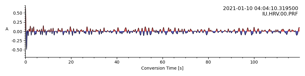
<AxesSubplot: xlabel='Conversion Time [s]', ylabel='A    '>

Let’s zoom into the first 20 seconds (~200km)

rftrace.plot(lim=[0,20])

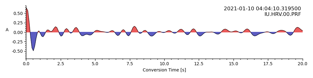
<AxesSubplot: xlabel='Conversion Time [s]', ylabel='A    '>

Plot RF section

Since we have an entire stream of receiver functions at hand, we can plot a section

rfstream.plot(scalingfactor=1)

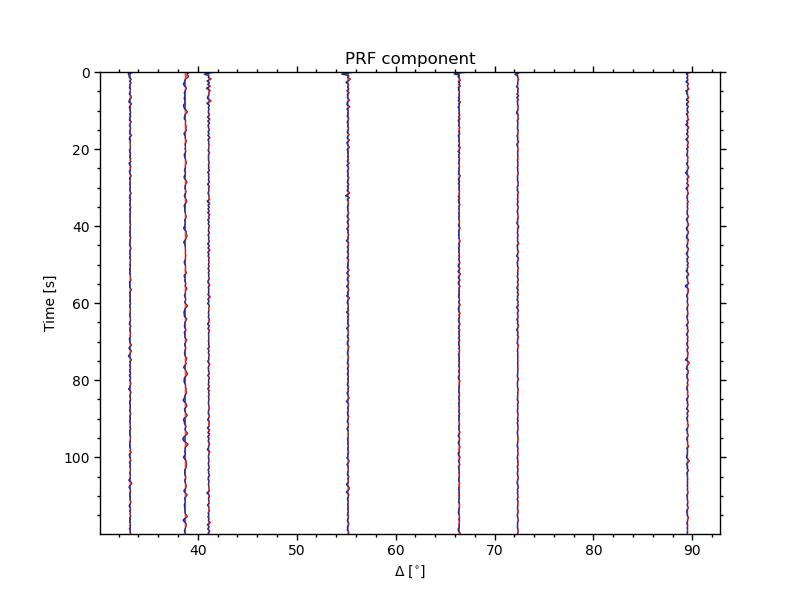
<AxesSubplot: title={'center': 'PRF component'}, xlabel='$\\Delta$ [$^{\\circ}$]', ylabel='Time [s]'>

Similar to the single RF plot we can provide time and epicentral distance limits:

timelimits = (0, 20)  # seconds
epilimits = (32, 36)  # epicentral distance
rfstream.plot(
    scalingfactor=0.25, lim=timelimits, epilimits=epilimits,
    linewidth=0.75)

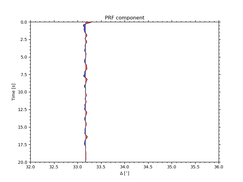
<AxesSubplot: title={'center': 'PRF component'}, xlabel='$\\Delta$ [$^{\\circ}$]', ylabel='Time [s]'>

By increasing the scaling factor and removing the plotted lines, we can already see trends:

rfstream.plot(
    scalingfactor=0.5, lim=timelimits, epilimits=epilimits,
    line=False)

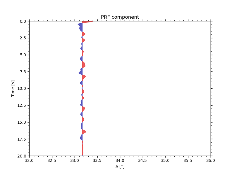
<AxesSubplot: title={'center': 'PRF component'}, xlabel='$\\Delta$ [$^{\\circ}$]', ylabel='Time [s]'>

As simple as that you can create your own receiver functions with just a single smalle script.