Note

Go to the end to download the full example code

Import from Local DataBase#

This Tutorial illustrates how to import waveform data from a local database of continuous waveforms into PyGLImER.

As we don’t have actual offline data available, we will download some continuous data from two stations: station IU-HRV ([Adam Dziewonski Observatory](http://www.seismology.harvard.edu/hrv.html)) and the Dutch station NL-HGN.

This data will then be sliced into times, when arrivals from teleseismic events are expected, which PyGLiMER determines in a previous step.

Downloading Event Catalogue & Feed in offline data#

Here, we will again use the pyglimer.waveform.request.Request class. The first method from this class that we are going to use is the download event catalog public method pyglimer.waveform.request.Request.download_evtcat(), to get a set of events that contains all wanted earthquakes. This method is launched automatically upon initialization. (Same as in the download tutorials)

To initialize said class we set up a parameter dictionary, with all the needed information. Let’s look at the expected information:

# sphinx_gallery_thumbnail_number = 1
# sphinx_gallery_dummy_images = 1

First let’s get a path where to create the data.

# Some needed Imports
import os
from typing import List
from obspy import UTCDateTime, read, read_inventory
import obspy
from pyglimer.waveform.request import Request

# Get notebook path for future reference of the database:
try: db_base_path = ipynb_path
except NameError:
    try: db_base_path = os.path.dirname(os.path.realpath(__file__))
    except NameError: db_base_path = os.getcwd()

# Define file locations
proj_dir = os.path.join(db_base_path, 'tmp', 'database_sac_import')


request_dict = {
    # Necessary arguments
    'proj_dir': proj_dir,
    'raw_subdir': os.path.join('waveforms', 'raw'),# Directory of the waveforms
    'prepro_subdir': os.path.join('waveforms', 'preprocessed'),  # Directory of the preprocessed waveforms
    'rf_subdir': os.path.join('waveforms', 'RF'),  # Directory of the receiver functions
    'statloc_subdir': 'stations', # Directory stations
    'evt_subdir': 'events',       # Directory of the events
    'log_subdir': 'log',          # Directory for the logs
    'loglvl': 'DEBUG',          # logging level, for more info use 'INFO' or 'DEBUG'
    'format': 'sac',              # Format to save database in
    "phase": "P",                 # 'P' or 'S' receiver functions
    "rot": "RTZ",                 # Coordinate system to rotate to
    "deconmeth": "waterlevel",    # Deconvolution method
    "starttime": UTCDateTime(2021, 1, 10, 3, 0, 0), # Starttime of your data.
    "endtime": UTCDateTime(2021, 1, 10, 5, 0, 0), # Endtimetime of your data
    # kwargs below
    "pol": 'v',                   # Source wavelet polaristion. Def. "v" --> SV
    "minmag": 5.0,                # Earthquake minimum magnitude. Def. 5.5
    "event_coords": None,         # Specific event?. Def. None
    "evtcat": None,               # If you have already downloaded a set of
                                  # events previously, you can use them here
}

Now that all parameters are in place, let’s initialize the pyglimer.waveform.request.Request

# Initializing the Request class and downloading the data
R = Request(**request_dict)

2023-03-29 10:32:48,905 - INFO - Successfully obtained 1 events

The initialization will look for all events for which data is available. To see whether the events make sense we plot a map of the events:

import matplotlib.pyplot as plt
from pyglimer.plot.plot_utils import plot_catalog
from pyglimer.plot.plot_utils import set_mpl_params

# Setting plotting parameters
set_mpl_params()

# Plotting the catalog
plot_catalog(R.evtcat)

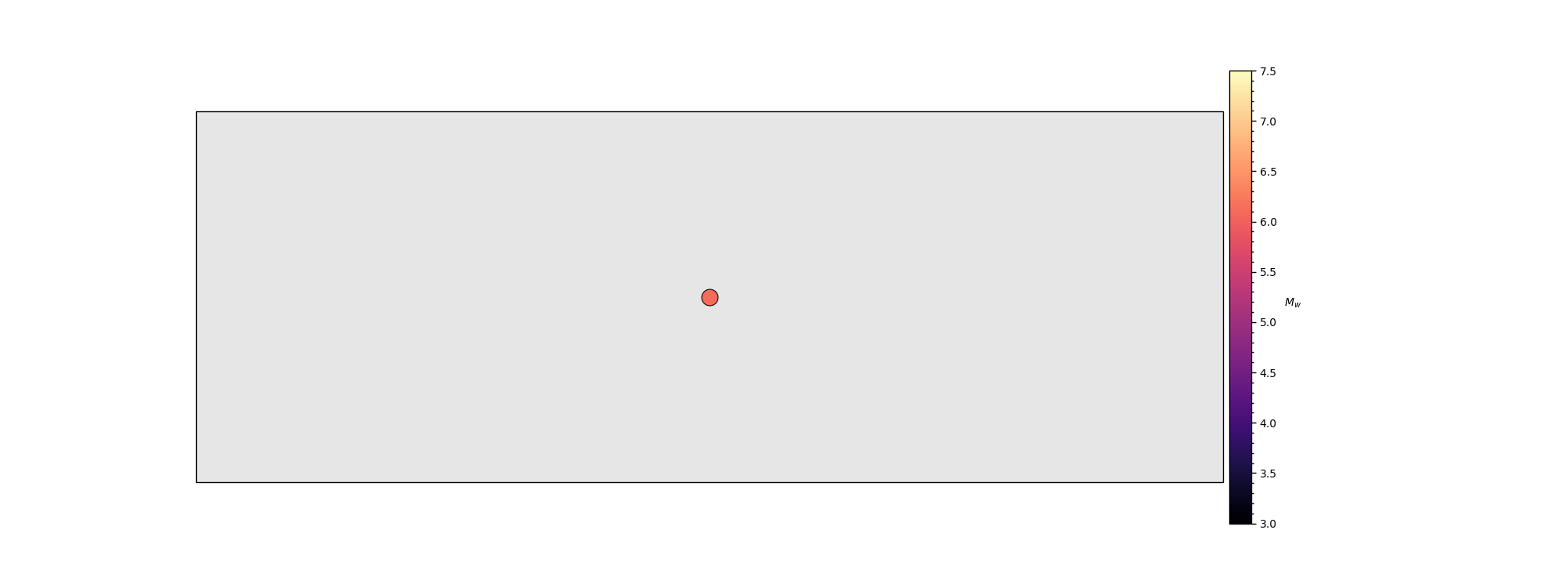
We can also quickly check how many events we gathered.

print(f"There are {len(R.evtcat)} available events")

There are 1 available events

Preliminary steps#

This will be the most complex step because it requires you to write two functions: 1. A function that yields Obspy Streams. 2. A function that yields obspy inventories.

*WARNING:* both have to yield information for the same station. So both Generators also need to have the same length.

These functions could for example look like this:

def yield_st_dummy(list_of_waveform_files: List[os.PathLike]):
    for file in list_of_waveform_files:
        yield obspy.read(file)


def yield_inventory_dummy(list_of_station_files: List[os.PathLike]):
    for file in list_of_station_files:
        yield obspy.read_inventory(file)

*NOTE:* This also requires you to convert/compile your information Into formats that obspy can read. To create StationXMLs follow the following tutorial: https://docs.obspy.org/tutorial/code_snippets/stationxml_file_from_scratch.html The StationXML needs to contain the following information: 1. Network and Station Code 2. Latitude, Longitude, and Elevation 3. Azimuth of Channel/Location to do the Rotation. 4. (Optional/if you set remove_response=True) Station response information.

The header of the traces need to contain the following: 1. sampling_rate 2. start_time, end_time 3. Network, Station, and Channel Code (Location code arbitrary) To convert seismic data from unusual formats to mseed or sac, we recommend using PyROCKO or obspy.

We will use two hours of data that come with PyGLImER

def yield_st():
    static = os.path.join(
        db_base_path, 'static_data', 'database_sac', 'waveforms', 'local_db')
    networks = ['IU']
    stations = ['HRV']
    for net, stat in zip(networks, stations):
        st = read(os.path.join(static, net, stat, 'hrv10.mseed'))
        yield st


def yield_inv():
    static = os.path.join(
        db_base_path, 'static_data', 'database_sac', 'waveforms', 'local_db')
    networks = ['IU']
    stations = ['HRV']
    for net, stat in zip(networks, stations):
        st = read_inventory(os.path.join(static, net, stat, 'hrv_stat.xml'))
        yield st

Import waveform data and station information#

The hard part is done! The actual import into PyGLImER is easy now: To do so, we use the public method of Request: import_database() This method will do the following: 1. Find times with teleseismic arrivals of our desired phase. 2. Slice time windows around this arrivals. 3. Do a first fast preprocessing. 4. Save Traces and station information in desired format (mseed or asdf)

R.import_database(yield_st, yield_inv)

2023-03-29 10:32:49,190 - INFO - Computing theoretical times of arrival. Save Inventories
2023-03-29 10:32:49,198 - INFO - Checking IU.HRV
2023-03-29 10:32:49,198 - DEBUG - IU.HRV
2023-03-29 10:32:49,221 - INFO - Slice data in chunks and save them into PyGLImER database.

Let’s just check how many teleseismic arrivals were found in this one week.

from glob import glob

# Path to the where the miniseeds are stored
data_storage = os.path.join(
    proj_dir, 'waveforms', 'raw', 'P', '**', '*.mseed')

# Print output
print(f"Number of found teleseismic arrivals: {len(glob(data_storage))}")

Number of found teleseismic arrivals: 1

*NOTE* From here on, the steps are identical to the download tutorials The final step to get you receiver function data is the preprocessing. Although it is hidden in a single function, which is pyglimer.waveform.request.Request.preprocess() A lot of decisions are being made:

Processing steps: 1. Clips waveform to the right length (tz before and ta after theorethical arrival.) 2. Demean & Detrend 3. Tapering 4. Remove Instrument response, convert to velocity & simulate havard station 5. Rotation to NEZ and, subsequently, to RTZ. 6. Compute SNR for highpass filtered waveforms (highpass f defined in qc.lowco) If SNR lower than in qc.SNR_criteria for all filters, rejects waveform. 7. Write finished and filtered waveforms to folder specified in qc.outputloc. 8. Write info file with shelf containing station, event and waveform information. 9. (Optional) If we had chosen a different coordinate system in rot than RTZ, it would now cast the preprocessed waveforms information that very coordinate system. 10. Deconvolution with method deconmeth from our dict is perfomed.

It again uses the request class to perform this. The if __name__ ... expression is needed for running this examples

R.preprocess(hc_filt=1.5, client='single')

2023-03-29 10:32:49,245 - INFO -


...Preprocessing initialiased...

2023-03-29 10:32:49,245 - DEBUG - USING SINGLE CORE BACKEND

  0%|          | 0/1 [00:00<?, ?it/s]2023-03-29 10:32:49,246 - INFO - Processing waveforms for event smi:service.iris.edu/fdsnws/event/1/query?eventid=11363293.
2023-03-29 10:32:49,262 - DEBUG - Before cut and resample
2023-03-29 10:32:49,263 - DEBUG -    Time elapsed: 0.0 s
2023-03-29 10:32:49,288 - INFO - Stream accepted. Preprocessing successful
2023-03-29 10:32:49,288 - INFO - File preprocessed.
Station IU.HRV
Event smi:service.iris.edu/fdsnws/event/1/query?eventid=11363293
2023-03-29 10:32:49,288 - DEBUG -    Time elapsed: 0.0 s
2023-03-29 10:32:49,300 - INFO - RF created.
Station IU.HRV
Event: smi:service.iris.edu/fdsnws/event/1/query?eventid=11363293
2023-03-29 10:32:49,300 - DEBUG -    Time elapsed: 0.0 s

100%|##########| 1/1 [00:00<00:00, 17.48it/s]
2023-03-29 10:32:49,303 - INFO - Preprocessing finished.

First Receiver functions#

The following few section show how to plot

Single raw RFs
A set of raw RFs
A move-out corrected RF
A set of move-out corrected RFs

Read the IU-HRV receiver functions as a Receiver function stream#

Let’s read a receiver function set and see what it’s all about! (i.e. let’s look at what data a Receiver function trace contains and how we can use it!)

from pyglimer.rf.create import read_rf

path_to_rf = os.path.join(proj_dir, 'waveforms','RF','P','*','*','*.sac')
rfstream = read_rf(path_to_rf)

print(f"Number of RFs: {len(rfstream)}")

Number of RFs: 1

PyGLImER is based on Obspy, but to handle RFs we need some more attributes:

from pprint import pprint

rftrace = rfstream[0]
pprint(rftrace.stats)

Stats({'sampling_rate': 10.0, 'delta': 0.1, 'starttime': UTCDateTime(2021, 1, 10, 4, 4, 10, 319538), 'endtime': UTCDateTime(2021, 1, 10, 4, 6, 40, 319538), 'npts': 1501, 'calib': 1.0, 'network': 'IU', 'station': 'HRV', 'location': '00', 'channel': 'PRF', 'sac': AttribDict({'delta': 0.1, 'depmin': -0.49419916, 'depmax': 0.6758249, 'scale': 1.0, 'b': 0.000538, 'e': 150.00053, 'o': -595.836, 'a': 29.97507, 'stla': 42.5064, 'stlo': -71.5583, 'stel': 200.0, 'evla': -24.0412, 'evlo': -66.5729, 'evdp': 217000.0, 'mag': 6.1, 'user1': 6.337349, 'baz': 175.01988, 'gcarc': 66.419815, 'depmen': -2.0729383e-05, 'nzyear': 2021, 'nzjday': 10, 'nzhour': 4, 'nzmin': 4, 'nzsec': 10, 'nzmsec': 319, 'nvhdr': 6, 'npts': 1501, 'iftype': 1, 'iztype': 9, 'leven': 1, 'lpspol': 1, 'lovrok': 1, 'lcalda': 0, 'kstnm': 'HRV', 'khole': '00', 'kuser0': 'time', 'kuser1': 'P', 'kcmpnm': 'PRF', 'knetwk': 'IU'}), '_format': 'SAC', 'station_latitude': 42.5064, 'station_longitude': -71.5583, 'station_elevation': 200.0, 'event_latitude': -24.0412, 'event_longitude': -66.5729, 'event_depth': 217000.0, 'event_magnitude': 6.1, 'event_time': UTCDateTime(2021, 1, 10, 3, 54, 14, 483001), 'onset': UTCDateTime(2021, 1, 10, 4, 4, 40, 294071), 'type': 'time', 'phase': 'P', 'distance': 66.419815, 'back_azimuth': 175.01988, 'slowness': 6.337349})

First Receiver function plots#

If the Receiver functions haven’t been further processed, they are plotted as a function of time. A single receiver function in the stream will be plotted as function of time only. A full stream can make use of the distance measure saved in the sac-header and plot an entire section as a function of time and epicentral distance.

Plot single RF#

Below we show how to plot the receiver function as a function of time, and the clean option, which plots the receiver function without any axes or text.

from pyglimer.plot.plot_utils import set_mpl_params

# Plot RF
rftrace.plot()

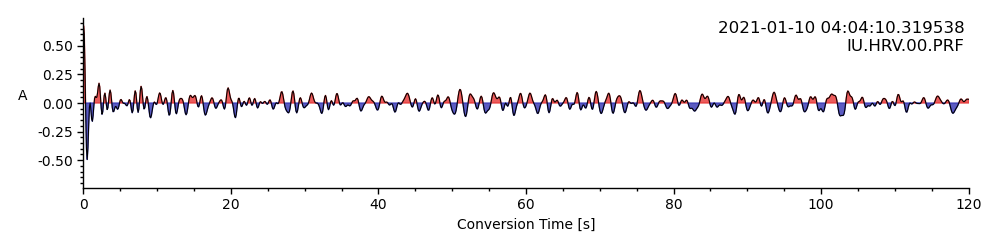
<AxesSubplot: xlabel='Conversion Time [s]', ylabel='A    '>

Let’s zoom into the first 20 seconds (~200km)

rftrace.plot(lim=[0, 20])

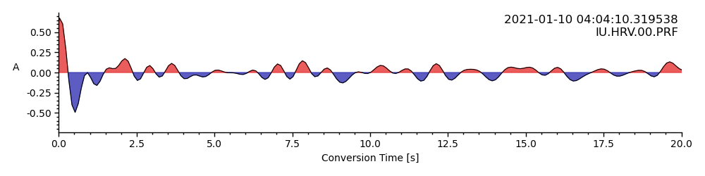
<AxesSubplot: xlabel='Conversion Time [s]', ylabel='A    '>

Plot RF section#

Since we have an entire stream of receiver functions at hand, we can plot a section

rfstream.plot(scalingfactor=1)

<AxesSubplot: xlabel='Conversion Time [s]', ylabel='A    '>

Similar to the single RF plot we can provide time and epicentral distance limits:

timelimits = (0, 20)  # seconds
epilimits = (32, 36)  # epicentral distance
rfstream.plot(
    scalingfactor=0.25, lim=timelimits, epilimits=epilimits,
    linewidth=0.75)

<AxesSubplot: xlabel='Conversion Time [s]', ylabel='A    '>

By increasing the scaling factor and removing the plotted lines, we can already see trends:

rfstream.plot(
    scalingfactor=0.5, lim=timelimits, epilimits=epilimits,
    line=False)

<AxesSubplot: xlabel='Conversion Time [s]', ylabel='A    '>

As simple as that you can create your own receiver functions with just a single smalle script.

Total running time of the script: ( 0 minutes 1.844 seconds)

Gallery generated by Sphinx-Gallery