Common Conversion Point Stack of a Single Station

The following notebook carries you through how to get from a set of receiver functions of a single station to a 3D common conversion point (CCP) stack. As an example as in the previous notebooks, we again use IU-HRV as example station.

Note

It is assumed here that you have successfully computed the receiver functions from the DataCollection{SAC | HDF5}.py.

Load the Receiver functions

# sphinx_gallery_thumbnail_number = 1
# sphinx_gallery_dummy_images = 1

So, first load the receiver functions into a RFStream.

import os
import matplotlib.pyplot as plt
from pyglimer.rf.create import read_rf
from pyglimer.plot.plot_utils import set_mpl_params
set_mpl_params()

# Define the location of the database
databaselocation = os.path.join('static_data', 'database_sac')  # or "database_hdf5"

try: db_base_path = ipynb_path
except NameError:
    try: db_base_path = os.path.dirname(os.path.realpath(__file__))
    except NameError: db_base_path = os.getcwd()
databaselocation = os.path.join(db_base_path, databaselocation)

rfst = read_rf(os.path.join(
    databaselocation, 'waveforms', 'RF', 'P', 'IU', 'HRV', '*.sac'))

# Check traces
print("Number of loaded RFs: ", len(rfst))
rfst[0].plot()
plt.show(block=False)

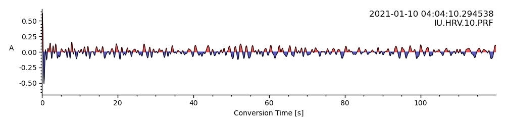
Number of loaded RFs:  7

Compute Common Conversion Point Stack

This is similar to the single station stacks.

from pyglimer.ccp import init_ccp
import os
import numpy as np

inter_bin_distance = 0.1
velocity_model = 'iasp91.dat'

ccp_init_dict = {
    'spacing': inter_bin_distance,
    'vel_model': velocity_model,
    "binrad": np.cos(np.radians(30)),
    "phase": 'P',
    "preproloc": os.path.join(databaselocation, "waveforms", "preprocessed"),
    "rfloc": os.path.join(databaselocation, "waveforms", "RF"),
    "network": "IU",
    "station": "HRV",
    "compute_stack": True,
    "save": 'ccp_IU_HRV.pkl',
    'format': 'sac',
    'mc_backend': 'joblib',
}

# Initialize bins
ccpstack = init_ccp(**ccp_init_dict)

  0%|          | 0/2 [00:00<?, ?it/s]
 50%|#####     | 1/2 [00:00<00:00,  6.41it/s]
100%|##########| 2/2 [00:00<00:00, 12.69it/s]

Finalizing the CCP Stack checking whether locations are on-land or not.

ccpstack.conclude_ccp(keep_water=True)

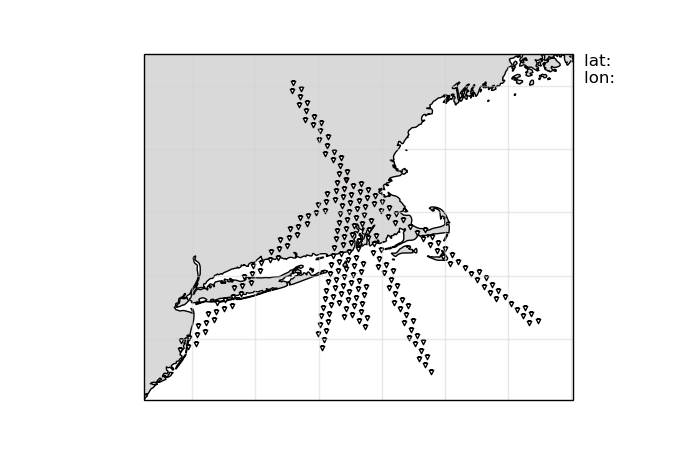
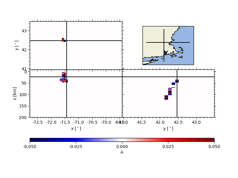
Plot Bins

import matplotlib.pyplot as plt
ccpstack.plot_bins()

Use the CCPStack object to image the subsurface

Given a CCPStack object there are multiple ways of getting an image of the subsurface. You could either compute a three-dimensional volume and plot slices with respect to the volume or you can create cross sections slices.

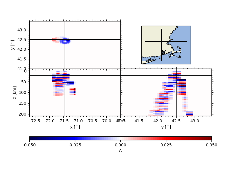
Compute a volume and slice

To do that we first need to read the created CCPStack. Second, we create a discretization for the are of interest, and third, we compute the volume and some slices.

import numpy as np
from pyglimer.ccp.ccp import read_ccp

# Reading the stack
ccpstack = read_ccp(filename='ccp_IU_HRV.pkl', fmt=None)

# Create discretization
lats = np.arange(41, 43.5, 0.05)
lons = np.arange(-72.7, -69.5, 0.05)
z = np.linspace(-10, 200, 211)

# Plotting the volume and slices
vplot = ccpstack.plot_volume_sections(
    lons, lats, zmax=211, lonsl=-71.45, latsl=42.5, zsl=23)

Creating Spherical Nearest Neighbour class ... done.
Creating interpolators ... done.
KDTree interpolation ... (intensive part)
KDTree interpolation ... (intensive part)--->  001/311
KDTree interpolation ... (intensive part)--->  032/311
KDTree interpolation ... (intensive part)--->  063/311
KDTree interpolation ... (intensive part)--->  094/311
KDTree interpolation ... (intensive part)--->  125/311
KDTree interpolation ... (intensive part)--->  156/311
KDTree interpolation ... (intensive part)--->  187/311
KDTree interpolation ... (intensive part)--->  218/311
KDTree interpolation ... (intensive part)--->  249/311
KDTree interpolation ... (intensive part)--->  280/311
KDTree interpolation ... (intensive part)--->  311/311
... done.
Regular Grid interpolation ... (less intensive part) done.

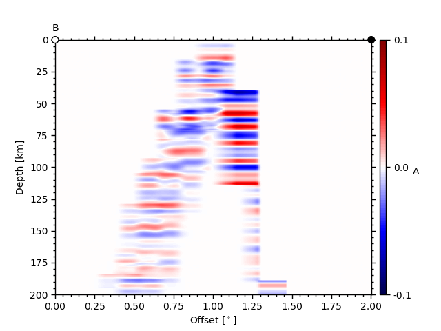
Slice CCPStack directly using

Here we first define two slices with their waypoints, and then plot a cross section in the back end, both RF sections and Illumination section are computed using a KDTree algorithm taking as input the CCPStack locations. For the illumination, this sometimes leads to weird results; see profile A

# Create points waypoints for the cross section
lat0 = np.array([42.5, 42.5])
lon0 = np.array([-72.7, -69.5])
lat1 = np.array([41.5, 43.5])
lon1 = np.array([-71.45, -71.45])

# Set RF boundaries
mapextent=[-73.5, -69, 41, 44]
depthextent=[0, 200]
vmin = -0.1
vmax =  0.1

# Plot cross sections
ax1, geoax = ccpstack.plot_cross_section(
    lat0, lon0, ddeg=0.01, z0=23, vmin=vmin, vmax=vmax,
    mapplot=True, minillum=1, label="A",
    depthextent=depthextent,
    mapextent=mapextent)
ax2, _ = ccpstack.plot_cross_section(
    lat1, lon1, ddeg=0.01, vmin=vmin, vmax=vmax,
    geoax=geoax, mapplot=True,
    minillum=1, label="B",
    depthextent=depthextent)
plt.show(block=False)

• 
• 
• 

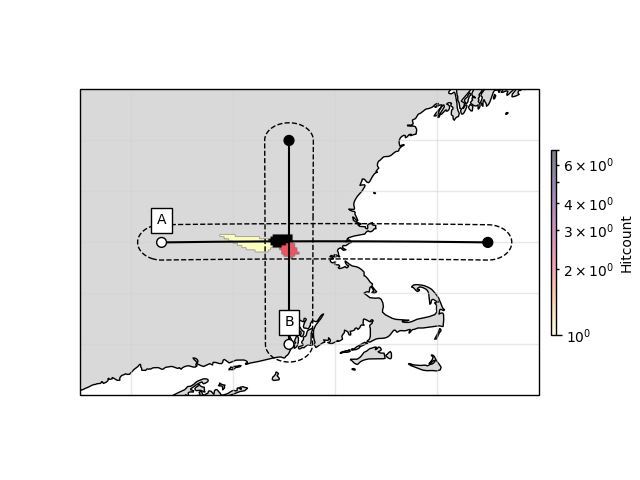
Note that here we are only running the example only with a very limited dataset, for which CCP Stacking makes limited sense. It still gives you an idea on how you could do this for a larger area. z0 here is the depth of the illumination map and minillum the minimum number of hitpoints per bin to be counted.

Note

The waypoints do not have to be just start and endpoint, they can be a series of points.

Compute a “dirty” global stack

In short, we are assuming that latitudes and longitudes are cartesian entities, with a small correction for the area of each bin that depends on the change in metric width of a degree of longitude as a function of latitude. This really is a dirty way of interpolation because the spherical nature of the Earth is disregarded.

We first read the RFs needed for the computation

from pyglimer.rf.create import read_rf
from pyglimer.plot.plot_utils import set_mpl_params
set_mpl_params()

rfst = read_rf(f"{databaselocation}/waveforms/RF/P/IU/HRV/*.sac")

Then, we migrate the receiver functions, i.e., move-out correct the RFs wrt. to a given model

z, rfz = rfst.moveout(vmodel='iasp91.dat')

and, compute the CCP volume like a 3D histogram by providing the extent of the region of interest, and dlon, which describes the longitudinal spacing.

Note

The latitudinal spacing is automatically computed.

# Set extent=[minlon, maxlon, minlat, maxlat]
extent = [-72.7, -69.5, 41, 43.5]

# Compute Dirty Stack
latc, lonc, zc, ccp, illum = rfz.dirty_ccp_stack(dlon=0.075, extent=extent)

Then, we can use the 3D histogram to plot the stack using the same tool as the ‘clean’ stacking.

from pyglimer.plot.plot_volume import VolumePlot

vp = VolumePlot(lonc, latc, zc[:211], ccp[:,:,:211], xl=-71.45, yl=42.5, zl=23)
plt.show(block=False)